How to Make CPU Cloth Simulation Fast
This post is about the work I did during my 8 week Summer of Code internship at Traverse Research where I worked on a cloth simulation system for the Breda framework. I had the limitations set for me that it had to run on the CPU, on a single thread and the goal of reaching a step time of < 0.5 ms per 10k-vertex garment at 60 Hz. I implemented vertex pinning so that cloths can be attached to other world objects such as character bones, collision with capsules and planes, self collision and integrated the solver into an ECS so separate cloth instances can have different parameters.
To achieve this performance goal I used ISPC kernels for hot paths with graph colouring my constraints, implemented Long Range Attachments to be able to reduce substep count and also simulating a separate coarse mesh and skinning the dense one on top of it to improve performance.
The Pipeline at a Glance
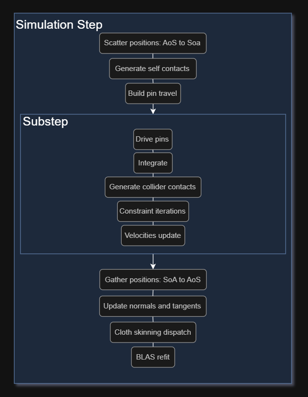
The basis of my solver is an XPBD solver, which itself is an extension of Position Based Dynamics. Positions are first converted into a structure of arrays layout once per step so that the kernels do unit stride loads. Self collision contacts are also found once per step against the whole steps displacement and then frozen throughout all the substeps if collision is predicted to occur. Colliders and pins are also interpolated across the substeps so that fast moving colliders sweep through the cloth instead of teleporting inside of it and that the pins don’t yank the cloth after themselves with big jumps every substep.
Inside of a substep I integrate my vertices and predict where they should be based on their velocities, then check for collider contacts, project all the constraints then derive the new velocities from how far the positions actually moved.
After completing all substeps I again convert my positions back to an array of structures, update all the vertex normals and tangents for rendering, skin the dense cloth mesh on top of the coarse one if there is one and then lastly refit the BLAS of my cloth.
XPBD and Small Steps
The reason to use XPBD rather than plain PBD is that in PBD, stiffness depends on the iteration count. Project a distance constraint 5 times and you get soft fabric, project it 50 times and you get sheet metal. That means every time you change the solver budget, you have to retune every piece of clothing in the game.
XPBD fixes this by giving each constraint a compliance and carrying a running Lagrange multiplier, so the constraint converges to a fixed physical stiffness regardless of how many iterations you throw at it. The compliance gets folded into the update as alpha_tilde = compliance / dt².
Here is the actual distance-constraint kernel, which is the clearest place to see the whole update at once:
foreach (i = batch_offsets[batch] ... batch_offsets[batch + 1]) {
    const int a = idx_a[i];
    const int b = idx_b[i];
    const float w_a = w_a_arr[i];
    const float w_b = w_b_arr[i];
    const float w_sum = w_a + w_b;

    const vec3 pa = { pos_x[a], pos_y[a], pos_z[a] };
    const vec3 pb = { pos_x[b], pos_y[b], pos_z[b] };
    const vec3 delta = pb - pa;
    const float dist = length3(delta);

    const bool active = w_sum != 0.0f && dist >= GEOM_EPS;
    const float mask = active ? 1.0f : 0.0f;

    // Positive when overstretched, negative when compressed.
    const float constraint = dist - rest_length[i];
    // `n` is the gradient of the constraint at `b`; `a` gets `-n`.
    const float inv_dist = 1.0f / (active ? dist : 1.0f);
    const vec3 n = delta * inv_dist;

    // `gamma` is uniform, so the whole gang skips the damping
    // gathers in the common undamped case.
    float damping = 0.0f;
    if (gamma != 0.0f) {
        const vec3 old_a = { old_x[a], old_y[a], old_z[a] };
        const vec3 old_b = { old_x[b], old_y[b], old_z[b] };
        damping = gamma * dot3(n, (pb - old_b) - (pa - old_a));
    }
    const float denom = (1.0f + gamma) * w_sum + alpha_tilde;
    const float delta_lambda = mask
        * (-(constraint + alpha_tilde * lambda[i] + damping)
            / (active ? denom : 1.0f));
    lambda[i] += delta_lambda;

    const vec3 corr_a = n * (-w_a * delta_lambda);
    pos_x[a] += corr_a.x; pos_y[a] += corr_a.y; pos_z[a] += corr_a.z;
    const vec3 corr_b = n * ( w_b * delta_lambda);
    pos_x[b] += corr_b.x; pos_y[b] += corr_b.y; pos_z[b] += corr_b.z;
}
The gamma term is Rayleigh damping, which resists the rate at which a constraint is being violated rather than the violation itself. It’s what stops a stiff sheet from ringing like a drum.
The second thing that matters is Small Steps in Physics Simulation. Given a fixed budget, you can spend it on more solver iterations inside one big step, or on more substeps each doing one iteration.
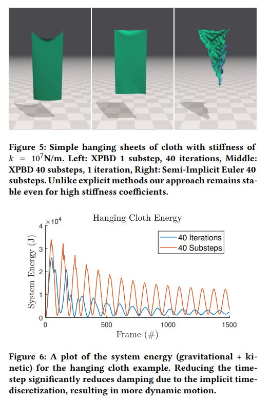
Substeps win, and not by a small margin because they result in significantly less stretching and better energy preservation shown in the picture above. The reason is the velocity update at the end of each substep, more iterations inside a single step just push positions around without ever letting the velocities catch up.
I also tried to implement Augmented Vertex Block Descent in an attempt to find some more performance, but after my initial implementation I measured the performance to be the same if not a bit worse than XPBD, which made more sense after reading Hallam Roberts writeup on their VBD implementation in Houdini where in the section about XPBD vs VBD performance they explain that VBD results in less graph colours but often doubles the amount of operations. So I decided to not put any more effort into that and stick with XPBD.
The Constraints

My cloth behaviour is derived from 6 types of constraints which are shown above. Stretch, shear, bending and tether constraints are all derived from the mesh when building the solver while the collider constraints are generated during each substep and self collision constraints are calculated per step.
They are solved from left to right and the order matters because we solve them Gauss-Seidel style, meaning each constraint updates positions in place and immediately feeds into the next, so later constraints in the sequence have the final say over earlier ones. This is why collider and self-collision constraints are solved last.
Stretch
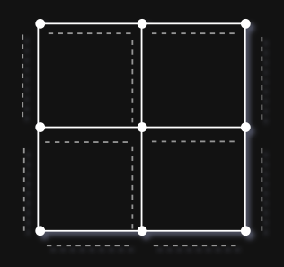
Stretch constraints are just a distance constraint on every structural edge, solved at its own compliance and damping using the kernel above.
Shear
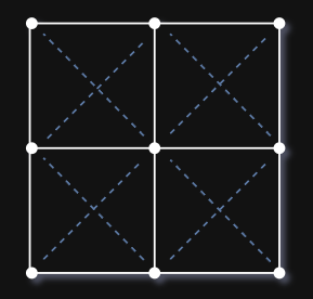
Shear constraints are a separate distance constraint class on the quad diagonals, solved at its own independent compliance. Splitting the two is what lets a fabric resist stretching along the weave while still shearing freely, which is most of what makes cloth look like cloth rather than rubber.
When an edge is a diagonal I add a shear constraint for it and also one for its mirror so the bracing is symmetric in both diagonal directions instead of only the one the triangulator happened to pick.
Bending
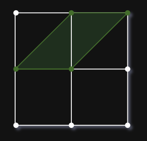
Bending constraints use the quadratic model from Bergou et al. 2006, one element per interior edge over that edge’s two vertices and the two opposite apexes. The weights are the cotangents of the angles opposite the edge, and they only depend on the rest pose, so they’re computed once when the solver is built:
// the cotangents of the angles at the shared edge's two endpoints, in each of the two adjacent triangles.
let cotangent = |corner: usize, to_a: usize, to_b: usize| -> Option<f32> {
    let (u, v) = (
        positions[to_a] - positions[corner],
        positions[to_b] - positions[corner],
    );
    let sin = u.cross(v).length();
    if sin > GEOM_EPS {
        Some(u.dot(v) / sin)
    } else {
        None
    }
};

let iso_weights = [-(c23 + c24), -(c13 + c14), c13 + c23, c14 + c24];
let rest_l: Vec3 = [p1, p2, p3, p4]
    .iter()
    .zip(iso_weights)
    .map(|(&p, k)| positions[p] * k)
    .sum();
Note the cotangent never calls a trig function. At solve time the constraint is C = ½(|L|² - rest) where L = Σ kᵢxᵢ, and the gradient at each vertex is just kᵢ · L:
const vec3 l = x1 * k1 + x2 * k2 + x3 * k3 + x4 * k4;
const float l_sq = dot3(l, l);
const float sum_wk2 = w1 * k1 * k1 + w2 * k2 * k2 + w3 * k3 * k3 + w4 * k4 * k4;
const float grad_sq = sum_wk2 * l_sq;

const float constraint = 0.5f * (l_sq - rest_l_sq_arr[i]);
// ... same XPBD update as the distance kernel ...

const float s1 = w1 * k1 * delta_lambda;
pos_x[p1] += l.x * s1;
pos_y[p1] += l.y * s1;
pos_z[p1] += l.z * s1;
// s2, s3, s4 the same way
So the whole element is dot products and multiplies. No dihedral angle, no acos, nothing that would stall a SIMD gang. It also makes no assumption about topology, which turns out to matter a lot for the coarse-mesh trick later on.
Tethers
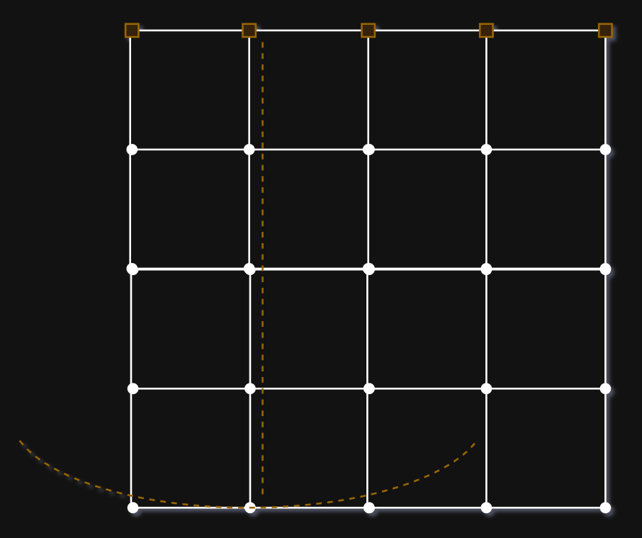
Tether constraints are optionally used at low iteration/substep counts to limit stretching. Even with well-tuned compliance, a sheet hanging under gravity stretches visibly. Position based methods propagate a correction one edge per iteration, so with a low iteration count the vertices near the bottom of a cape simply never hear about the pins at the top before the frame ends. Increasing iterations until it stops is exactly the cost we’re trying to avoid.
The fix is Long Range Attachments: give each free vertex a unilateral distance constraint straight to a pinned vertex, so it can never get further from that pin than it is in the rest pose. One constraint, no propagation needed, and because it’s unilateral it does nothing at all until the cloth is actually over-extended.
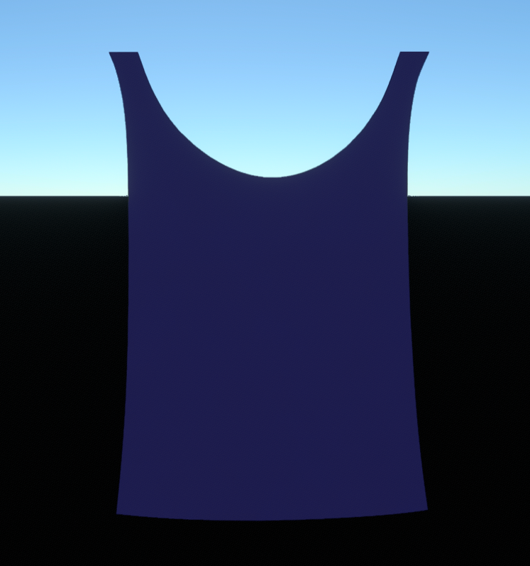
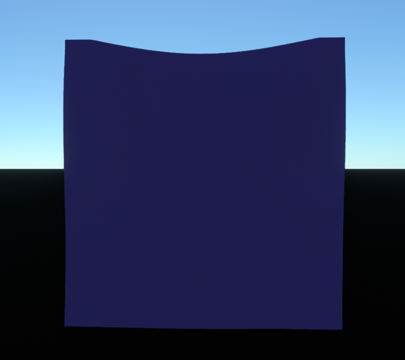
The two pictures below show tethers in action. Both pictures were taken with the solver set at 2 substeps and the same cloth but the second one has tethers enabled while the first one doesn’t.
Colliders
The collider set is deliberately small: capsules and planes. Capsules cover limbs, torsos and props well enough that a character is a handful of them, and the closest-point test against a capsule is cheap enough that I don’t run a broadphase at all. I also added planes to test out how dropping the cloth on the ground would react but I never got to make it look nice because the self collision wasn’t really reacting well under that stress of dropping the cloth, but more on that later.
Contact generation is swept. I’m not just checking for “is this vertex inside a capsule”, but I intersect the segment from the vertex’s old position to its predicted position against the capsule.
The projection ended up as three passes fused into one kernel, and each of them exists because of a specific failure I hit:
- A live analytic push-out against every capsule, not just the generated contacts, because the previously solved constraints can drag a vertex into a collider after generation ran, and a contact-driven solve leaves it sitting inside.
- The frozen swept entry plane, for a vertex that tunnelled all the way through inside one substep and is now genuinely outside on the far side, where a surface test can’t see it. The first version of this resolved such vertices toward the prediction side, which flipped the cloth to the wrong side of a limb.
- An unconditional half-space projection, last, so that when a plane and a capsule disagree the ground always wins.
Fused means one kernel, one load and one store per vertex, with p threaded through all three passes as a local:
foreach (i = 0 ... vertex_count) {
    if (inv_mass[i] == 0.0f) {
        continue;
    }
    vec3 p = { pos_x[i], pos_y[i], pos_z[i] };

    // Pass 1: live push-out against every capsule surface.
    for (uniform int j = 0; j < collider_count; ++j) {
        if (kind[j] != COLLIDER_CAPSULE) continue;
        // ... if p is inside, p = on_axis + nn * radius
    }

    // Pass 2: swept entry plane, only for this substep's hit slots.
    for (uniform int j = 0; j < collider_count; ++j) {
        if (kind[j] != COLLIDER_CAPSULE || hit[j * vertex_count + i] == 0) continue;
        // ... if the vertex tunnelled through, push it back across the entry plane
    }

    // Pass 3: half-spaces, last, so the ground wins.
    for (uniform int j = 0; j < collider_count; ++j) {
        if (kind[j] != COLLIDER_PLANE) continue;
        const float penetration = dot3(p - p0, u);
        if (penetration < 0.0f) {
            p = p - u * penetration;
        }
    }

    pos_x[i] = p.x;
    pos_y[i] = p.y;
    pos_z[i] = p.z;
}
Each kind[j] test is uniform, so the whole gang skips a collider of the wrong type rather than masking lanes off.
Friction and restitution happen at the velocity level, and restitution is hard zero. I also remove the whole normal component rather than reflecting any of it. That’s not physical, but keeping it ejects a vertex that penetrated by depth d at a speed of d/dt, that ejection fights the stretch constraints, and the result buzzes visibly. Removing it all looks far better.
Self Collision
I followed the predictive-contacts approach from Chris Lewin’s GDC 2018 talk, and the single structural decision that comes from it is that contacts are found once per step and then frozen for every substep and iteration underneath because detection is the expensive half and the solve is comparatively free. Three contact kinds run simultaneously and none of them knows about the others: point-point, vertex-triangle, and edge-edge (the last from Bridson et al.).
Contacts are also generated speculatively: a pair gets a contact if it’s already within the target distance, or if additive CCD says it’s closing fast enough to touch before the step is over.
Outside of that I also made some other choices:
Sweep bounds relative to the mean displacement. A cape moving coherently through the world would otherwise inflate every swept AABB by the character’s velocity. Taking the sweep relative to the mesh’s mean displacement means only genuine relative motion costs anything, and a cape being carried in a straight line generates almost no candidates.
Emitting each contact exactly once was the bulk of the implementation effort and none of it is in the paper. A shared vertex or edge belongs to several triangles, so the same feature pair gets discovered several times over. It took three mechanisms stacked: representative-triangle ownership so each shared feature is claimed by exactly one triangle, a lowest-overlapping-cell test so a pair straddling several cells is still emitted once, and canonical ordering on top of both. Neighbours within two rings are excluded outright.
Jacobi here, Gauss-Seidel everywhere else. Every other constraint type goes to some trouble to preserve exact sequential ordering. For self-contacts I gave that up. Each lane owns one vertex and reads from a frozen snapshot, so the result is independent of the SIMD width. It was cheaper and the ordering guarantee wasn’t worth anything here.
Vectorising a Gauss-Seidel Solve
Gauss-Seidel means each constraint reads what the last one wrote; if two constraints in the same SIMD gang share a vertex, they read and write the same address in the same instruction and you have a race.
Graph colouring fixes it. Colour the constraints so no two sharing a vertex get the same colour, then do one colour at a time. Within a colour every lane touches disjoint vertices, so the in-place scatter-accumulate is safe, and the result is bit-identical to running them sequentially.
fn greedy_color<const N: usize>(
    particles_per_constraint: impl Iterator<Item = [usize; N]>,
    vertex_count: usize,
) -> Vec<u32> {
    // Bitmask of colors taken per vertex; one word suffices below valence
    // 64, growing for pathological fans.
    let mut used: Vec<Vec<u64>> = vec![Vec::new(); vertex_count];
    particles_per_constraint
        .map(|particles| {
            let words = particles.iter().map(|&p| used[p].len()).max().unwrap_or(0);
            // Some word in 0..=words has a free bit: the word at `words` is
            // past the end of every particle's mask and thus all zero.
            let color = (0..=words)
                .find_map(|w| {
                    let occupied = particles
                        .iter()
                        .fold(0u64, |acc, &p| acc | used[p].get(w).copied().unwrap_or(0));
                    if occupied == u64::MAX { None }
                    else { Some(w as u32 * 64 + occupied.trailing_ones()) }
                })
                .unwrap();
            // ... mark `color` taken on every particle
            color
        })
        .collect()
}
Stable-sort the constraints by colour, keep the prefix offsets, and the kernels become a uniform outer loop over batches wrapping a vectorised inner loop:
for (uniform int batch = 0; batch < batch_count; ++batch) {
    foreach (i = batch_offsets[batch] ... batch_offsets[batch + 1]) {
        // every lane here touches disjoint vertices
    }
}
With the races gone, everything else was layout, and the theme is stop gathering:
- SoA positions, transposed once per step, so kernels do
pos_x[i]instead of strided3*ireads. - Per-constraint copies of the inverse masses.
inv_mass[idx_a[i]]is a gather; storingw_a[i]next to the constraint makes it a unit-stride load. Duplicating data to avoid an indirection feels wrong but measured clearly better. - Slot-major tether payloads with
-1sentinels, so each slot is unit-stride and the kernel canbreakwhenall(a < 0). - Masked arithmetic instead of branches, visible in the kernel above, inactive lanes compute something harmless and multiply it away rather than diverging.
uniformscalars to skip whole blocks, likegammaletting the entire gang skip the damping gathers when nothing is damped.
Simulating a Coarse Mesh and Skinning the Dense One
This is the change that mattered most and resulted in the most performance gain. Solver cost scales with simulated vertices while visual detail scales with rendered vertices. Up to this point the only lever I had for making a garment cheaper was making it look worse.
So the solver runs on a coarse mesh and the render mesh is bound to it, like skeletal skinning with a triangle mesh for a skeleton. Three ways to get the coarse mesh: the render mesh itself when it’s already cheap, an artist-authored coarse mesh baked out of the same glTF as a second mesh, or automatic meshopt simplification to a vertex budget using meshopt-rs.
Flat barycentric interpolation of a coarse mesh looks like a coarse mesh, so the surface gets reconstructed with Phong tessellation instead. Project the flat point onto each corner’s tangent plane and blend the three. Five lines on the CPU at bind time:
/// Must stay identical to the reconstruction in `cloth_skin.cs.hlsl`.
fn phong_surface_point(bary: [f32; 3], positions: [Vec3; 3], normals: [Vec3; 3]) -> Vec3 {
    let flat: Vec3 = (0..3).map(|i| bary[i] * positions[i]).sum();
    (0..3)
        .map(|i| bary[i] * (flat - normals[i] * (flat - positions[i]).dot(normals[i])))
        .sum()
}
and the same arithmetic again in the one compute shader this feature has:
// Phong tessellation, matching `phong_surface_point` in breda-cloth's sim_mesh.rs.
float3 position = float3(0, 0, 0);
for (uint i = 0; i < 3; i++) {
    float3 projected =
        flat - cornerNormals[i] * dot(flat - cornerPositions[i], cornerNormals[i]);
    position += weights[i] * projected;
}
Performance Results
The results are the mean time of one step, over around 240 frames, measured on an Intel i7-13650HX, in a scene with the cloth hanging and a capsule going back and forth colliding with it.
The coarse-mesh split is the headline. Every row renders the same 100x100 mesh at 2 substeps:
| Simulated vertices | Rendered vertices | Step time |
|---|---|---|
| 100x100 | 100x100 | 1.387 ms |
| authored 45×45 | 100x100 | 0.300 ms |
| simplified to 2000 | 100x100 | 0.281 ms |
Every row renders a 32x32 mesh at 20 substeps. The step column measures how much time a step takes excluding self collision detection and solve, and the detection and solve column show how long they take inside one step
| Self collision | Step | Detection | Solve |
|---|---|---|---|
| off | 0.946ms | - | - |
| on | 0.943ms | 2.166ms | 0.007ms |
Conclusion
The goal I was given was a step time under 0.5 ms for a 10k-vertex garment on a single CPU thread at 60 Hz. The final numbers are 0.300 ms with an artist-authored coarse mesh and 0.281 ms with automatic simplification, both of them still rendering the full 100x100 mesh, which is exactly that 10k-vertex garment. So the target was met with a bit of headroom left over.
Getting there happened in two fairly distinct phases, and only the second one actually closed the gap.
The first phase was making the solver I already had as fast as I could. ISPC kernels for every hot path, graph colouring so those kernels could run wide without racing, a structure of arrays layout, hunting down gathers and replacing them with unit-stride loads, and masked arithmetic instead of branches so lanes stop diverging. Together that took a 10k-vertex cloth from around 2.5 ms to about 1.3 ms. Half the cost for the same simulation, and I think all of it was worth doing.
What finally closed the gap wasn’t making each vertex cheaper, it was simulating fewer of them. Decoupling the simulated mesh from the rendered mesh dropped that same garment to 0.300 ms without changing anything the viewer sees.
Along the way the solver picked up what it needed to be used in a real scene rather than a demo. Pins can be driven by a character’s bones, so a cape hangs off a skeleton and gets its motion from the pins dragging the cloth after the body rather than from being carried:
Pins can also be changed at runtime, which is what lets something pull the cloth off its anchors and carry it away:
The cloth can also interact with the wind in the scene, sampled per vertex:
And the solver is driven through an ECS component, so every cloth instance in a scene carries its own parameters and can be authored in a world file instead of just in code:
Two things I’m not happy with about the Self collision. First is that its still very expensive. Detection alone costs over 2 ms on a 32x32 sheet, which is more than the entire budget for a garment several times that size. The structural win from the predictive-contacts approach is in there, but I never went back and chased the constant factor the way I did for the rest of the solver, so it stays off by default. Secondly the plane-drop case never got solid: dropping a cloth flat onto the ground puts a huge number of triangles into contact in the same step, and my self collision doesn’t hold up under that, which is why every demo here has the cloth hanging rather than piling up.
Further improvements
- Multithread the colour batches: the solver is still single-threaded. The constraints within a colour are already particle-disjoint, which is exactly the property a work-stealing split needs, so this is the obvious next win.
- A GPU path: the SoA layout and the colour batches map onto compute thread groups almost directly.
- Wrinkle maps: small-scale creases as a normal map driven by local strain, on top of the coarse solve.
- A simulation LOD: the sim/render split is already the mechanism, so driving the vertex budget from screen coverage is mostly plumbing.
- Better garment authoring: seam and sewing constraints so a garment can be built from flat panels, plus painted per-vertex weights. The weight plumbing already exists, it just has no tool in front of it.
References
-
[Müller et al. 2007] Position Based Dynamics: the paper the whole family of methods comes from.
-
[Macklin et al. 2016] XPBD: Position-Based Simulation of Compliant Constrained Dynamics: compliant constraints, which is what makes stiffness independent of the iteration count.
-
[Macklin et al. 2019] Small Steps in Physics Simulation: why substeps beat solver iterations at equal cost.
-
[Bergou et al. 2006] A Quadratic Bending Model for Inextensible Surfaces: the isometric bending model, no trig and no grid assumption.
-
[Kim et al. 2012] Long Range Attachments: stopping a hanging sheet from stretching without paying for more iterations.
-
Chris Lewin (GDC 2018) Cloth Self Collision with Predictive Contacts: the self-collision approach, and the reason detection runs once per step.
-
[Teschner et al. 2003] Optimized Spatial Hashing for Collision Detection of Deformable Objects: the broadphase.
-
[Li et al. 2021] Codimensional Incremental Potential Contact: additive CCD, used for speculative contact generation.
-
[Bridson et al. 2002] Robust Treatment of Collisions, Contact and Friction for Cloth Animation: edge-edge contact handling.
-
[Boubekeur & Alexa 2008] Phong Tessellation: reconstructing a smooth surface from a coarse mesh.
-
ISPC: the compiler that turns one kernel into six instruction sets.